Rotational speed and model
The rotational speed of the water wheels is logged over a long period of time and then used to create a model that creates a relationship between river parameter data and the speed.
Measurement module
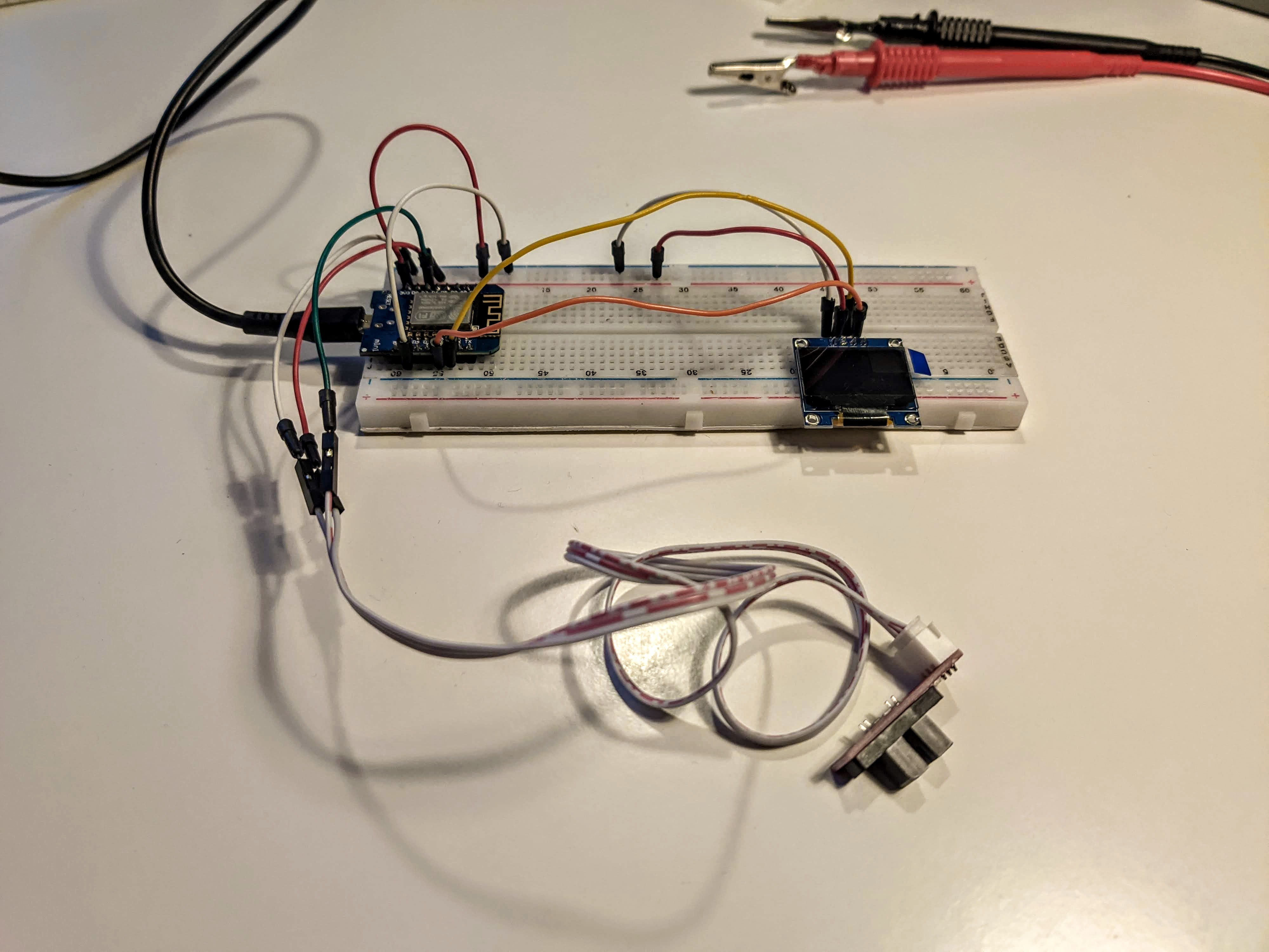
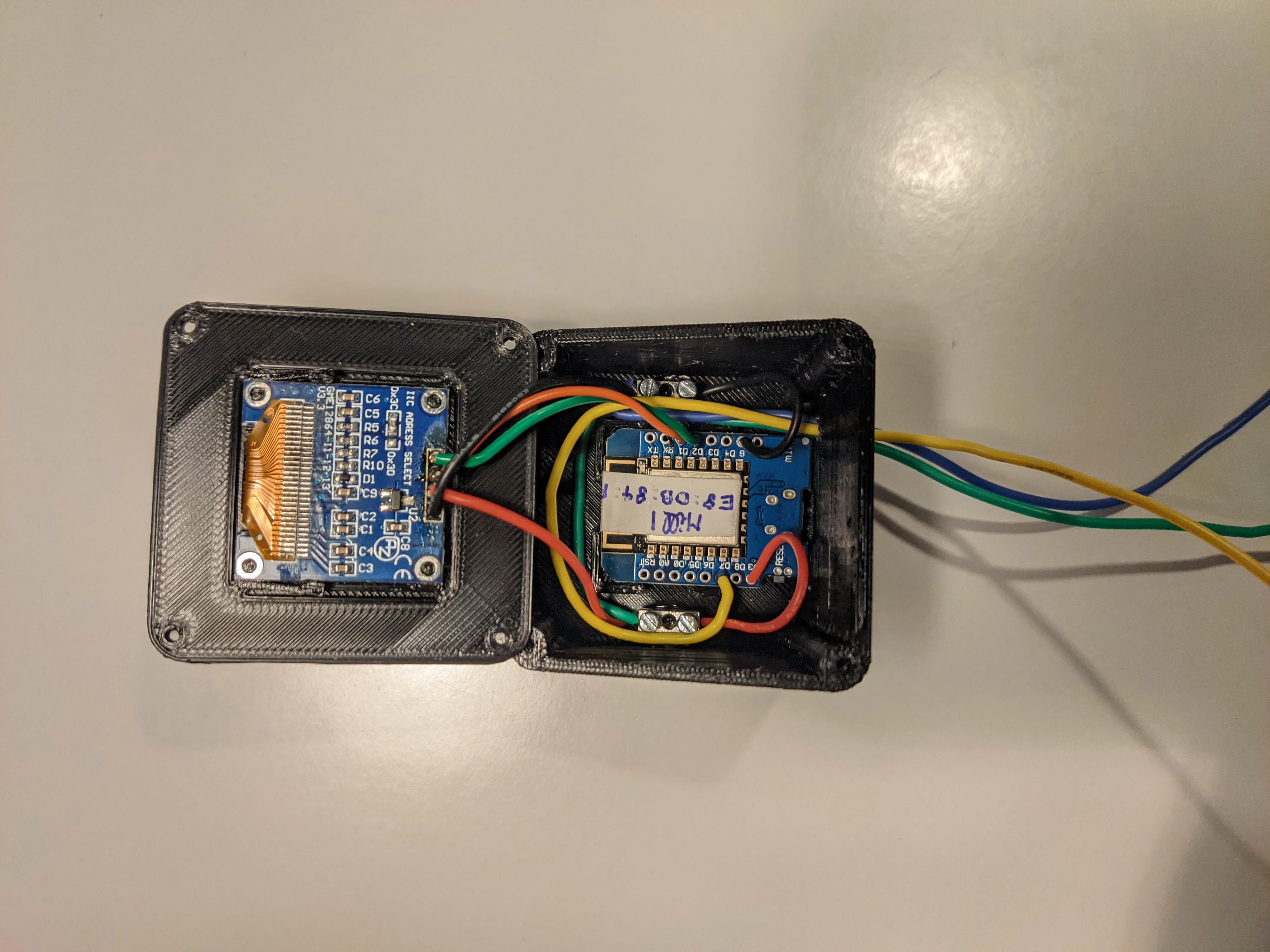
A custom measurement module was made to get the rotational speed of the watermills. This module sends every single RPM value to a Google spreadsheet through a webapp, which in turn is displayed by this website to provide real-time data. It contains the following hardware:
- 3D printed case
- D1 mini (ESP8266 microprocessor)
- OLED display
- Optical switch
Design and testing
The module was first tested thoroughly in a breadboard setup. The rotational speed is calculated using the time difference between two optical switch triggers. Then it is sent to the spreadsheet to ultimately be displayed on the OLED screen.
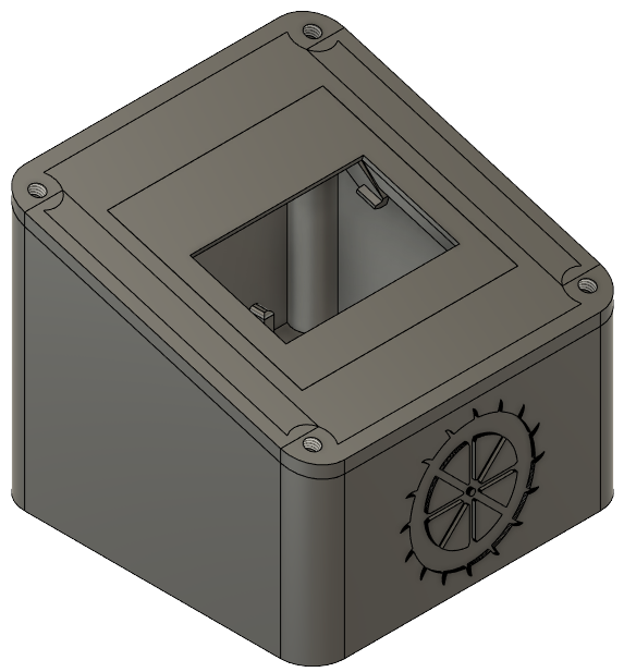
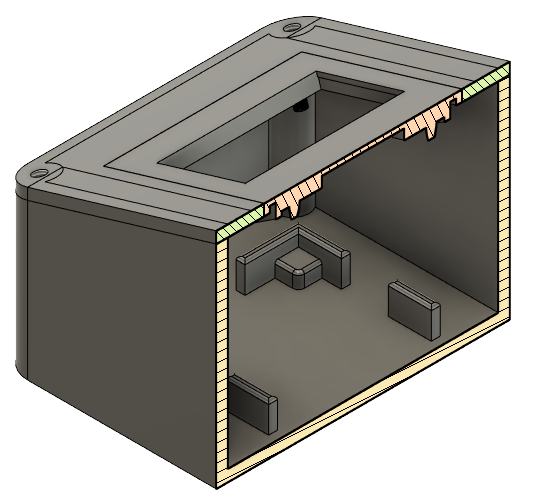
Then a case was designed using Fusion 360 and 3D printed.
Final result
Finally, the components were placed in the case and the module was installed inside the mill house.
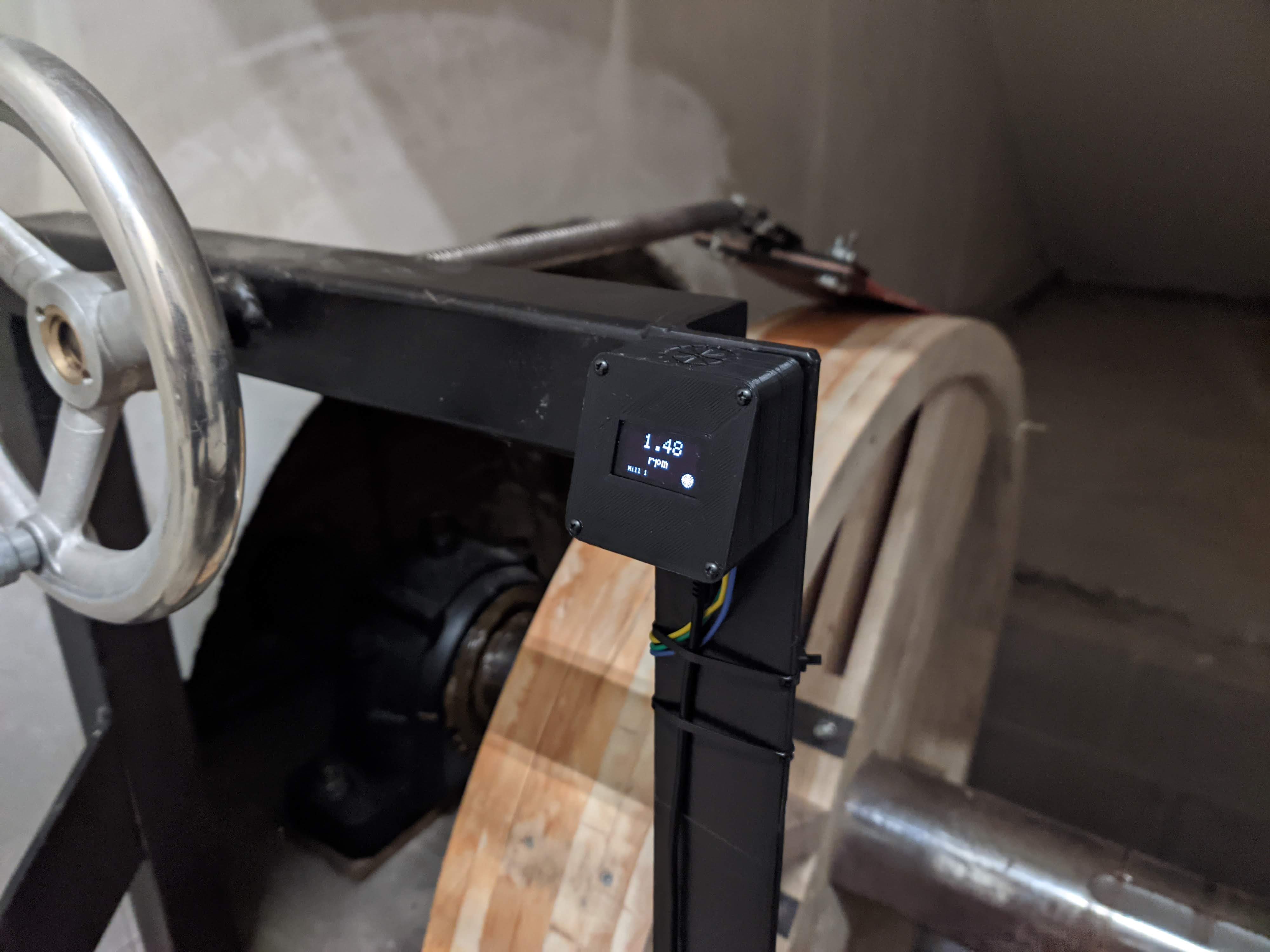
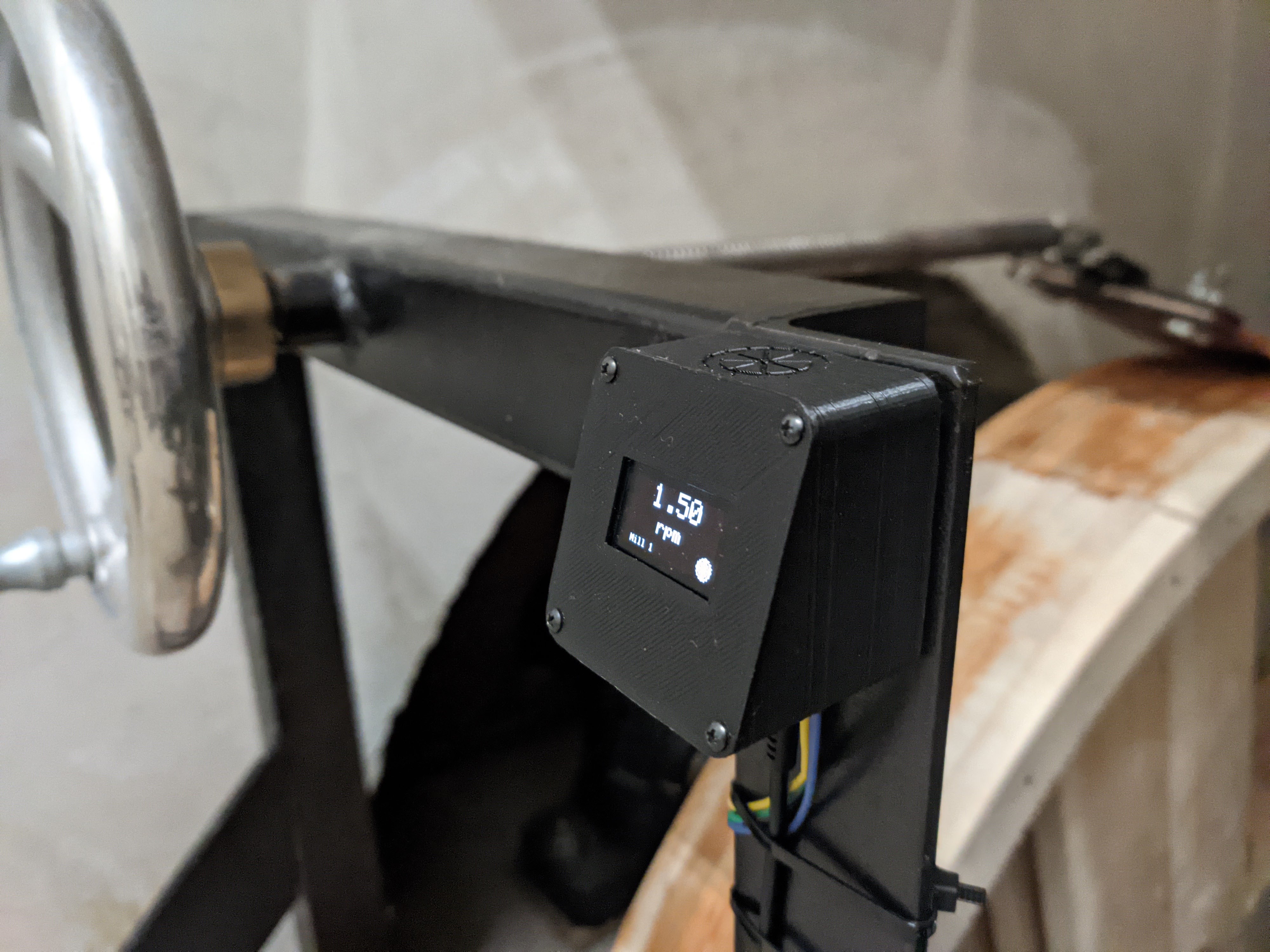
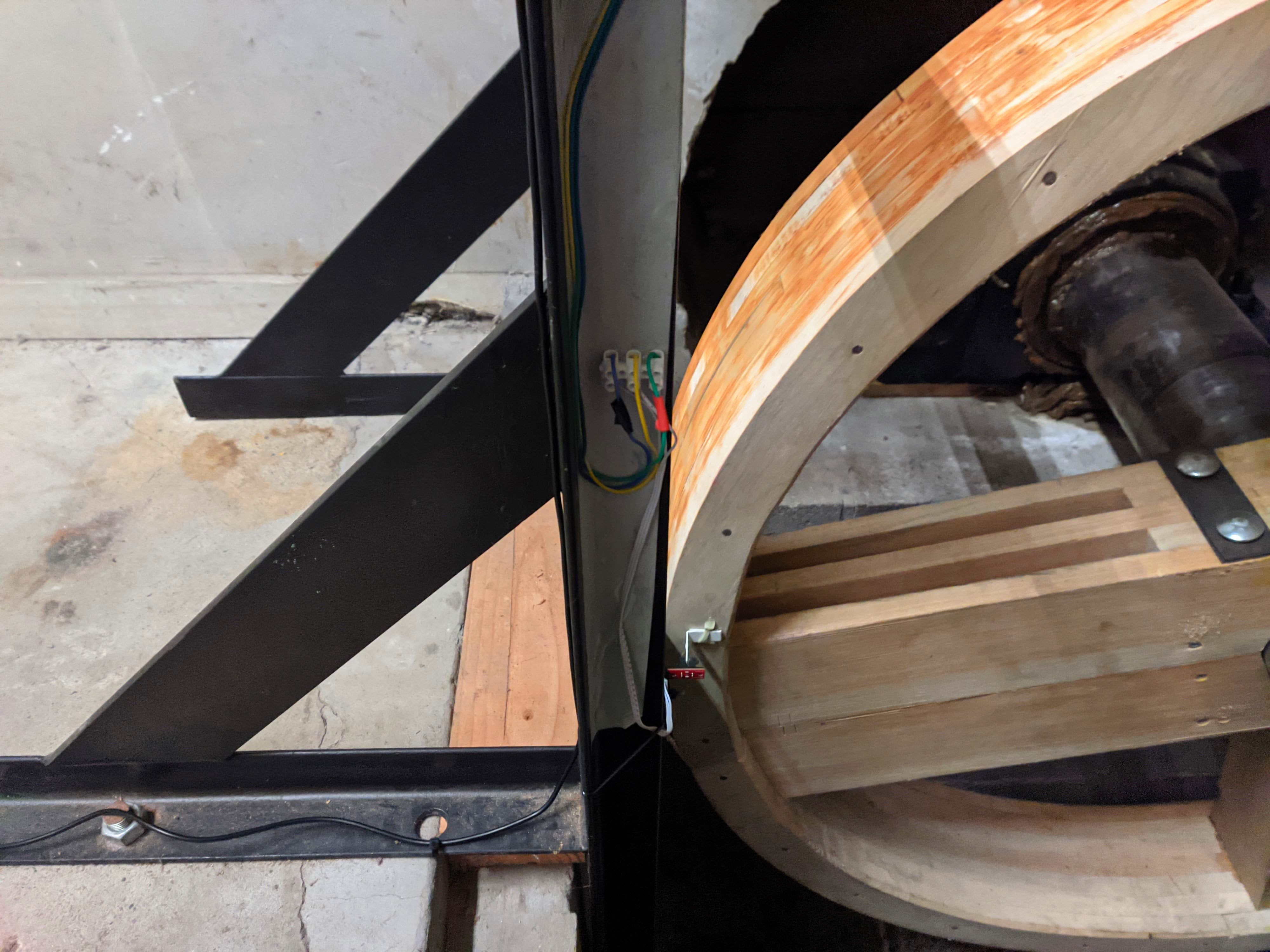
A piece of plastic is glued to the axis of the water wheel and passes through the optical switch to trigger it.
Model
Goal
To be able to properly estimate the energy production capacity of the mills, it is interesting to create a model of the rotational speed in terms of data that has been recorded over a longer time. This would allow us to go back in time and estimate the rotational speeds based of the other data. In the end, that allows us to do a financial feasibility analysis to answer the age old question: will the mills ever produce energy? Luckily for us, the VMM has been recording water level data at a station close to the mill since 2006.

Correlation data
Aligning this data with our own RPM measurements is the first step to finding a good model. The figure below shows the chronological course of water level data (source: VMM) and the measured RPM of both mills. There is clearly a relation between the two.
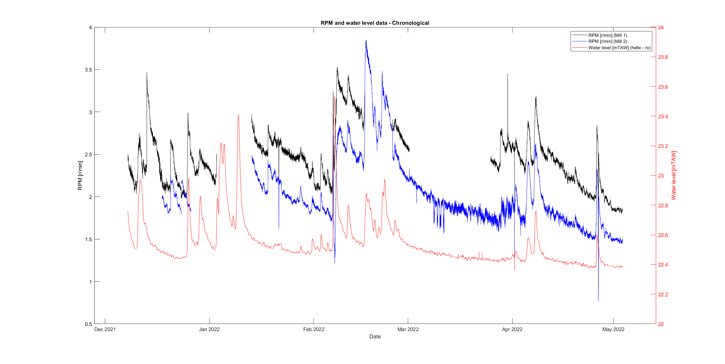
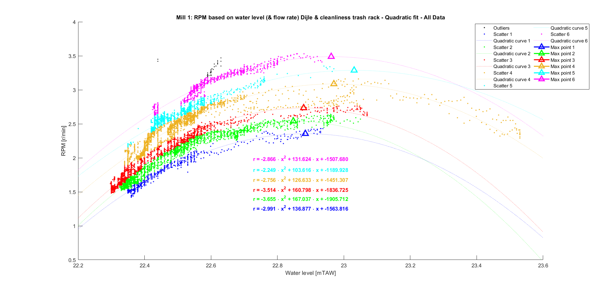
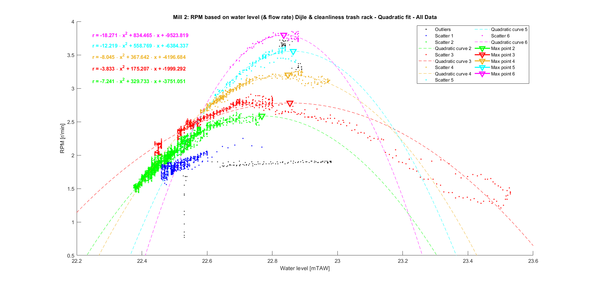
Plotting the RPM in function of the water level, shows this connection more clearly and reveals other insights. There are different ‘bins’ where the data can be put in, depending on the dirt build-up in trash rack placed before the water wheels.
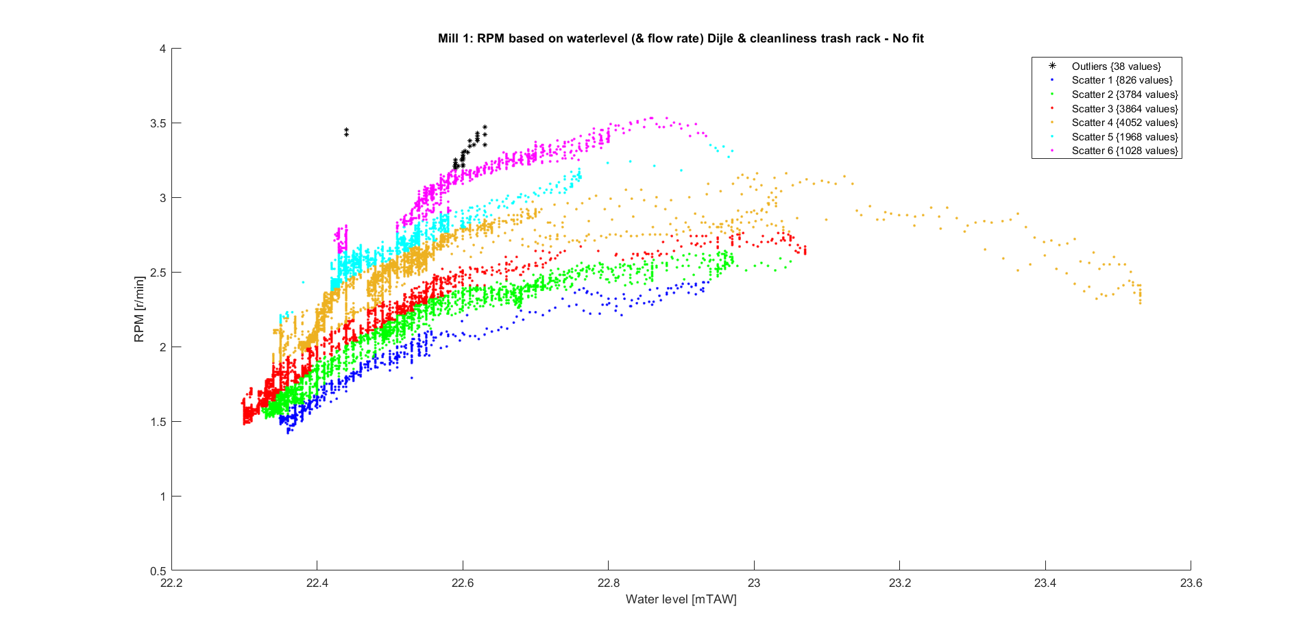
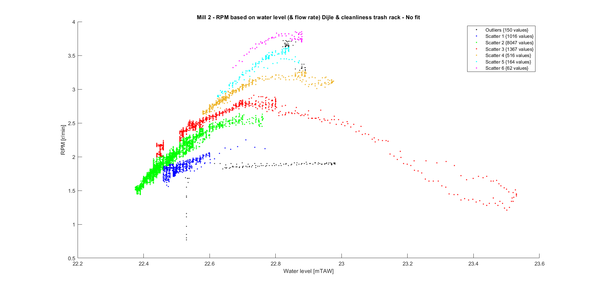
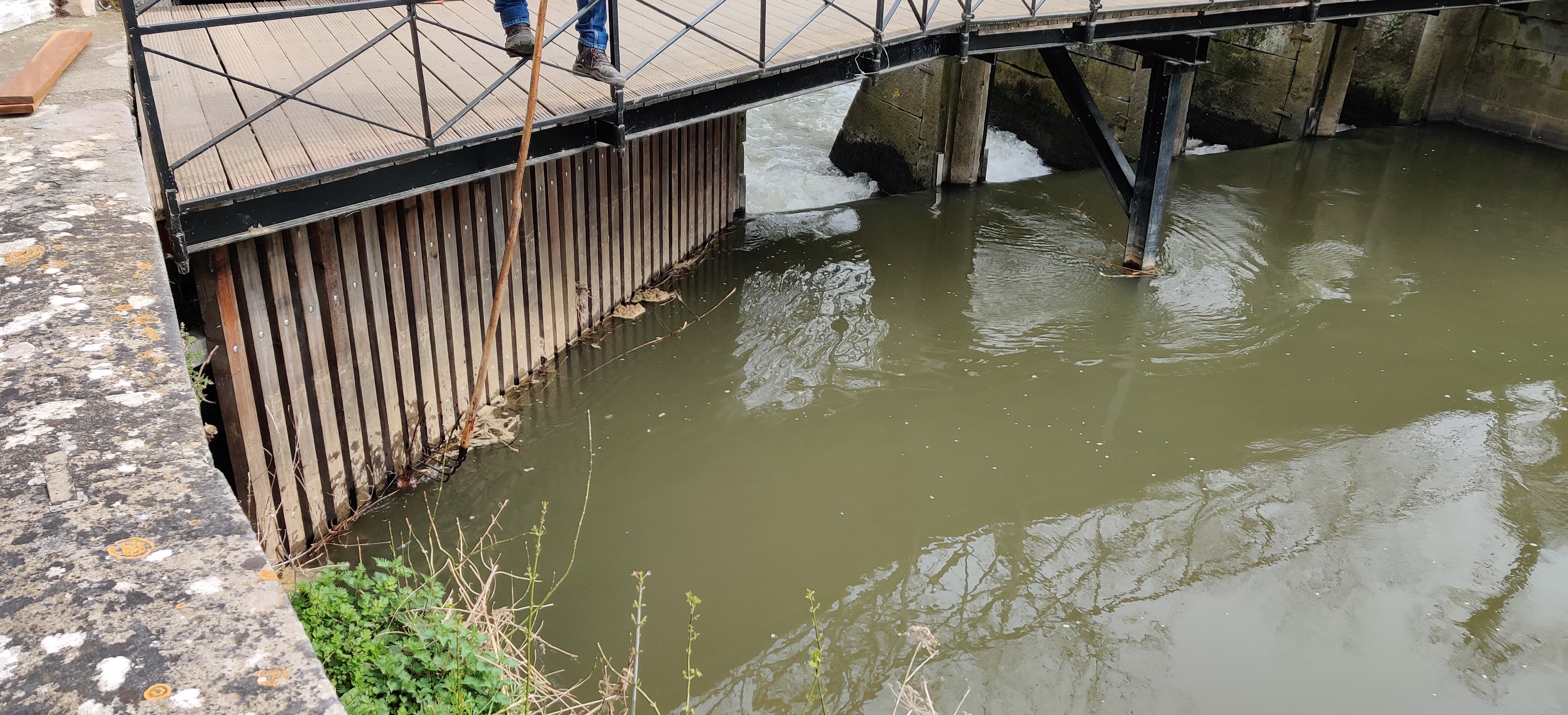
The trash rack gathers all the sediment, leafs, branches… and prevents the blades from being damaged. Their influence on the RPM is significant, as is their importance to prevent damage. However, making the gaps between the wooden planks larger would be beneficial for rotational speed, without letting too much trash in.
Curve fitting
Now the data bins have been found, fitting a curve to the most complete bin of every mill gives insight in the exact relation between the water level and the rotational speed.
Mill 1
A quadratic and cubic fit were performed on the data of mill 1.
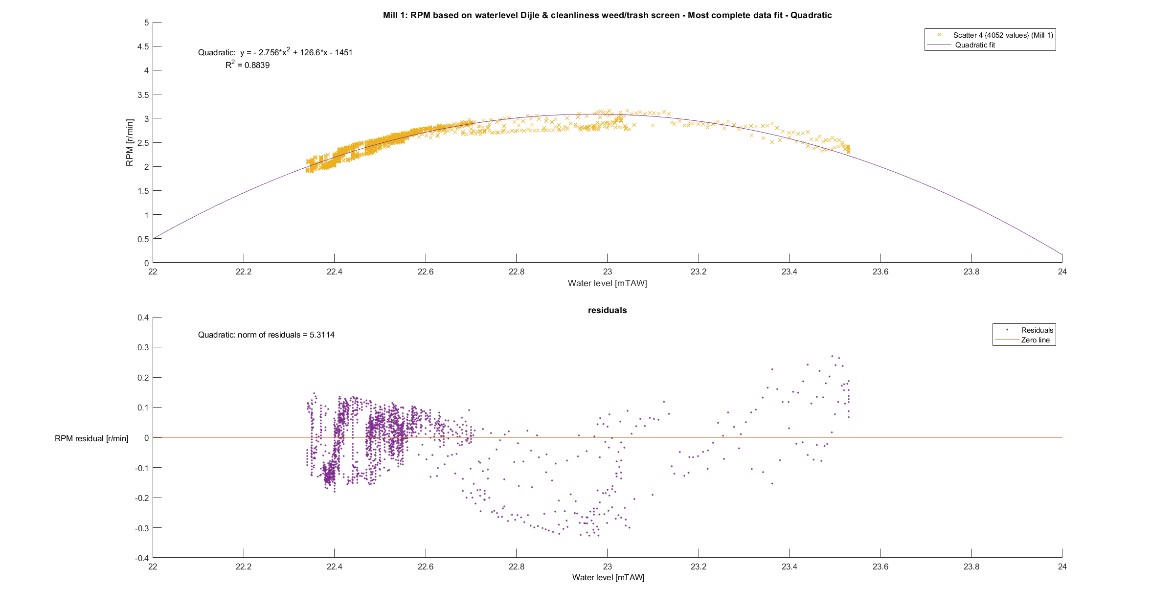
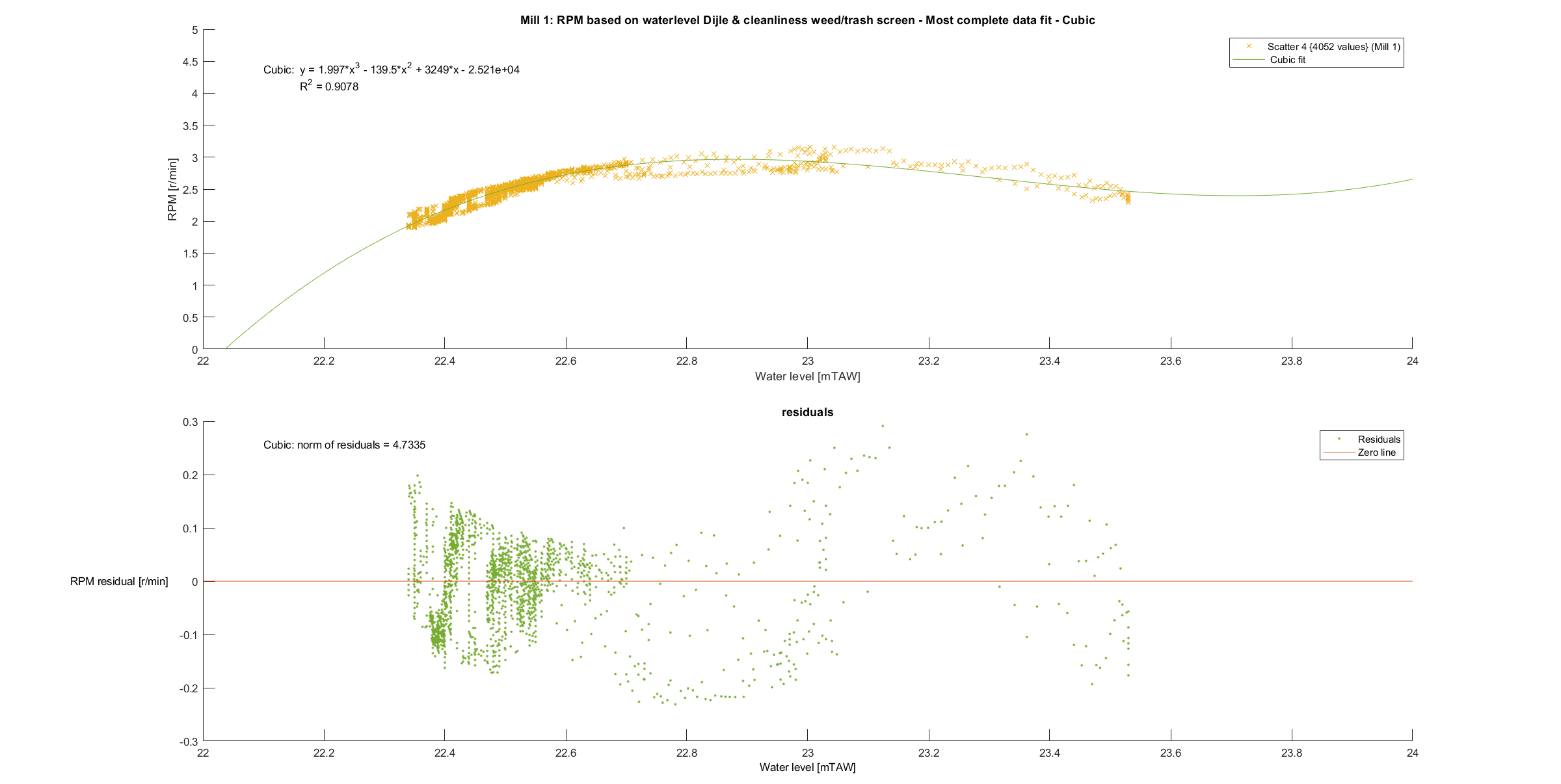
The cubic fit seems to fit the data better (higher R squared and more random residuals), but is badly conditioned. This means that there are large rounding errors in the process of fitting the curve. Small changes in the input (more data) therefore have a large influence in the output (the fitted curve). Unfortunately, getting more data for higher water levels is impossible. The measuring station prevents the water level from passing above a certain threshold to make sure the city is not flooded, see more here.
Intuitively, a quadratic model makes more sense too. Since there is no regulation of the water level at the watermill, a higher water level means that the water up- and downstream of the water wheels are almost equal. The kinetic energy of the flowing water is mostly what makes the wheels turn. A higher water level means more water hitting the blades upstream and thus transferring more kinetic energy to the blades. It also means there is more resistance downstream of the water wheel, because of the blades that have to push water up against the cruel grasp of gravity.
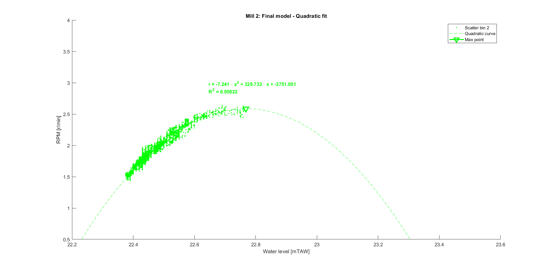
Mill 2
The same was done for mill 2.
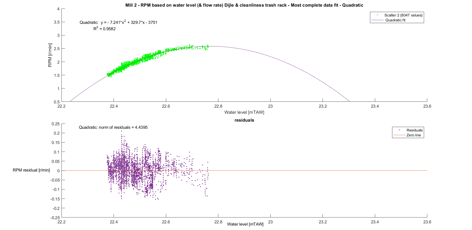
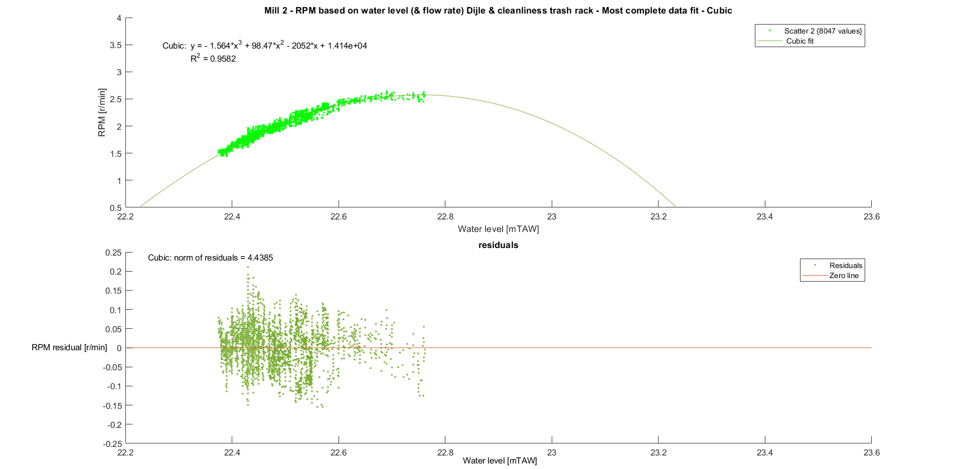
And the same results were found for this data.
Final model
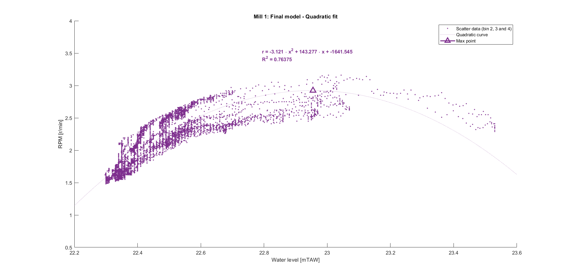
The final model is therefore a quadratic fit for both mills. Performing this on the other data bins yield the graphs listed below.
Now that the model of every bin is known, it is beneficial to select a single curve. This allows us to easily extrapolate the data later on, without running into a convoluted analysis of the estimated rpm for every bin. An option would be to use the fitted curve from the bin that contains the most data points. For mill 2, this makes a lot of sense as over 70% of the data points belong to the same bin. For mill 1, it is a bit more nuanced. The data points are more evenly distributed over the bins, but are mostly evenly distributed over bin 2, 3 and 4. Since their respective fitted curves are very similar in shape, they can be considered to be one and the same bin. This yields the following final equations and graphs:
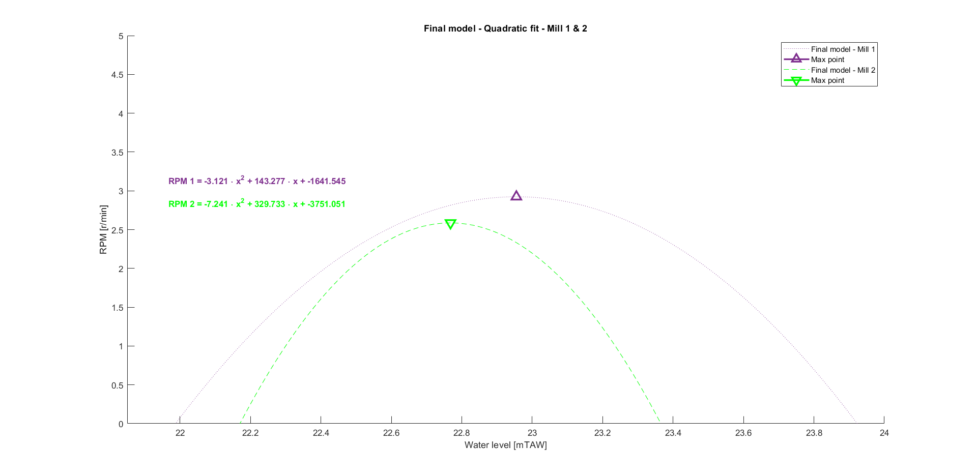
Relation mills
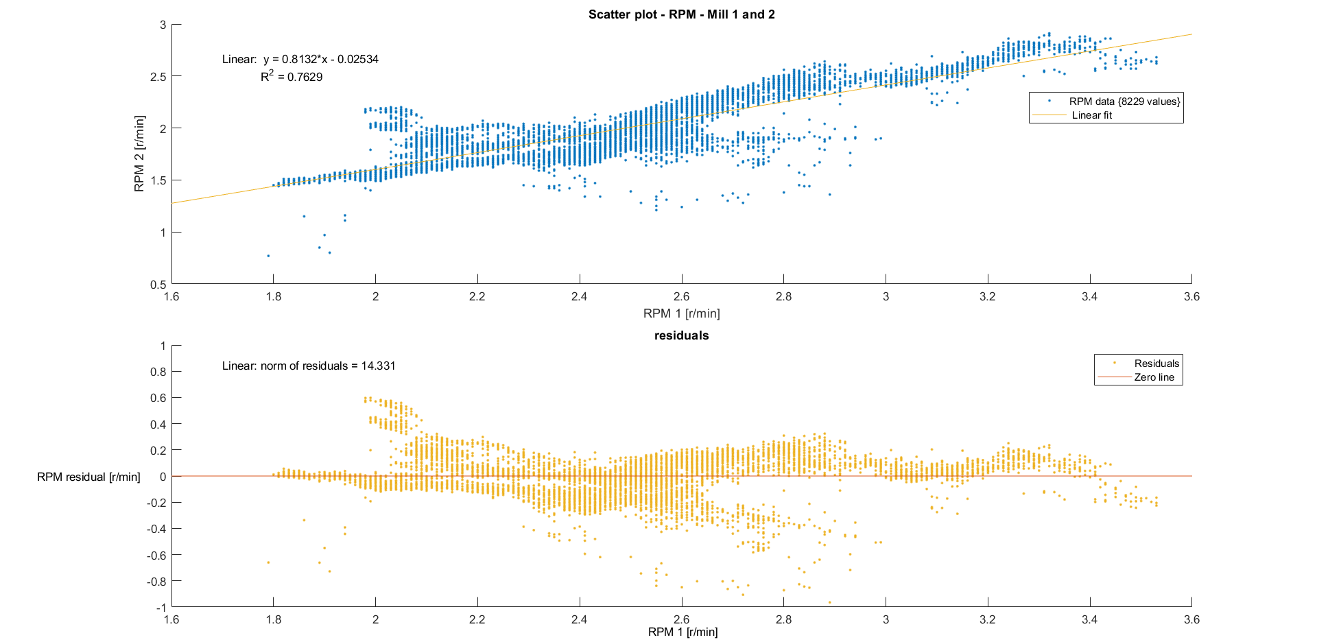
The keen observer might have wondered why the curves are not similar for corresponding bins between the mills. In other words: couldn’t we have just done the modelling for every bin of one mill to then transform this curve to the corresponding bin of the other mill? Both mills are designed exactly the same (so they should be roughly the same weight and have roughly the same center of gravity), are driven by the same river and just separated by a brick wall. Unfortunately, there seems to be no good linear connection between the rotational speeds of both mills. There seem to be some external factors (e.g. flow of water, wear on axis/blades…) which do not allow for a simple model.
Extrapolation
The next step is to extrapolate the rotational speed dating all the way back to 2006. The respective final model from before is used for every mill.
Mill 1
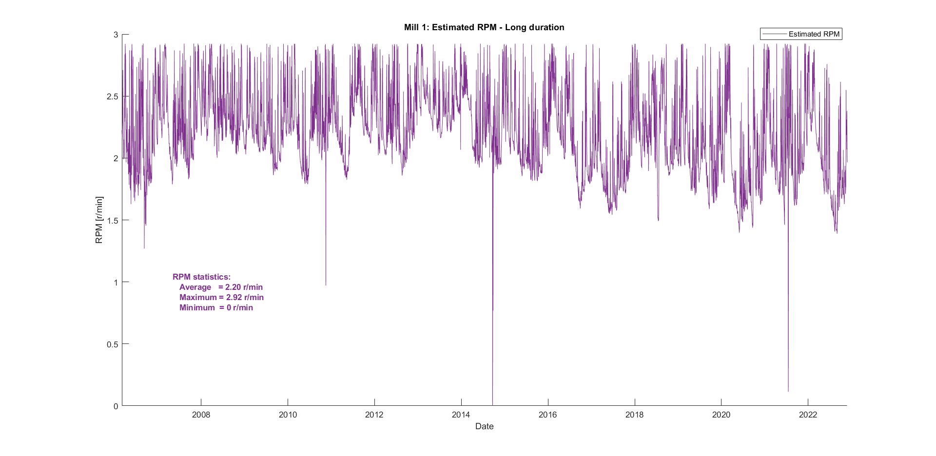
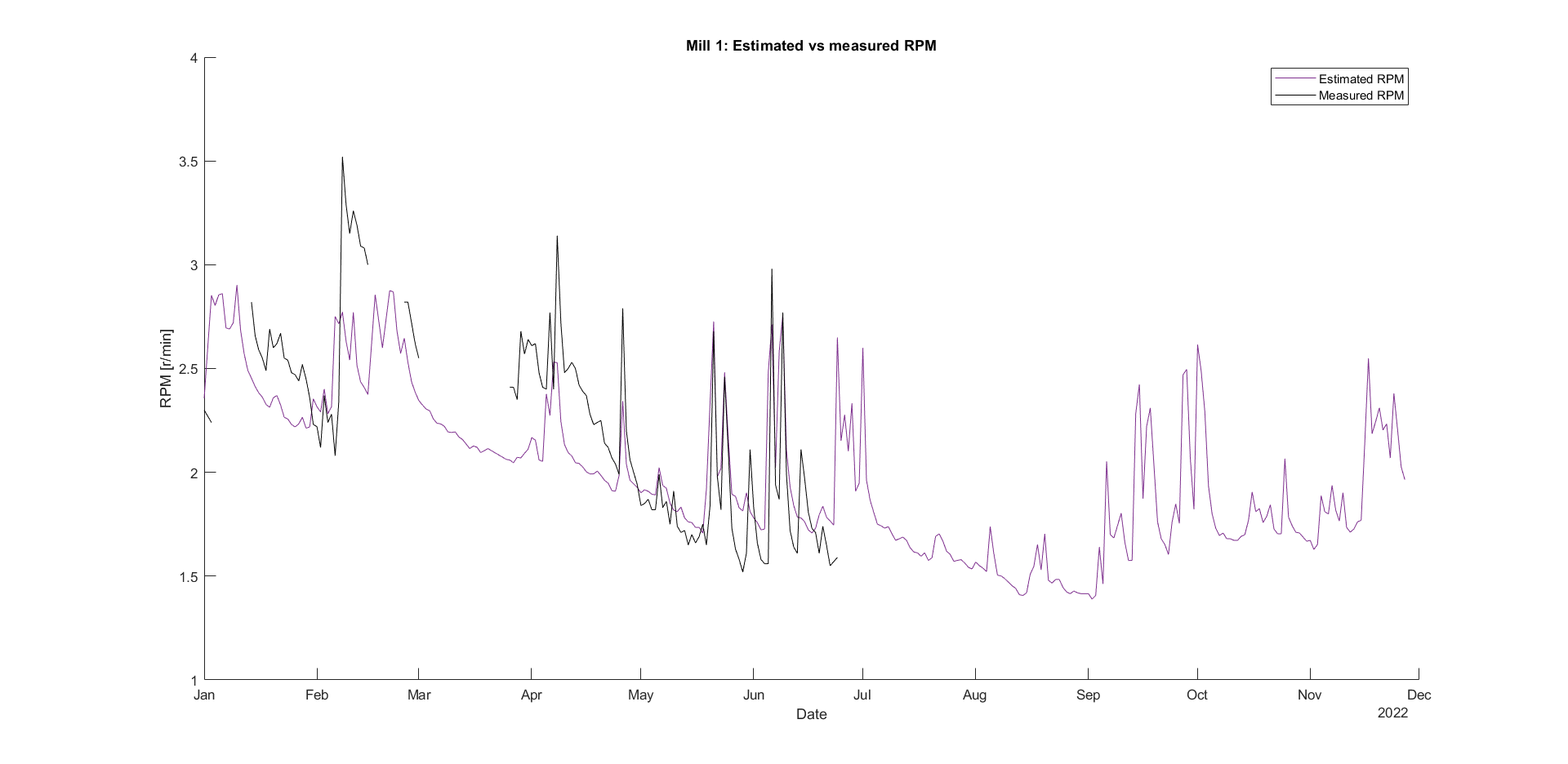
This view does not say much, but zooming to the year 2022 and comparing it to the actual measurements reveals how good the model is. The figure below shows that the model is sufficient for mill 1. Because there is no overpowering single bin, it was expected that the extrapolated curve would not fit the actual curve perfectly.
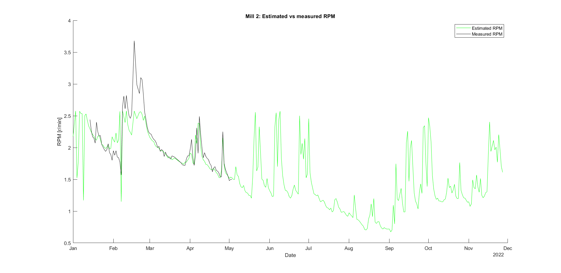
Mill 2
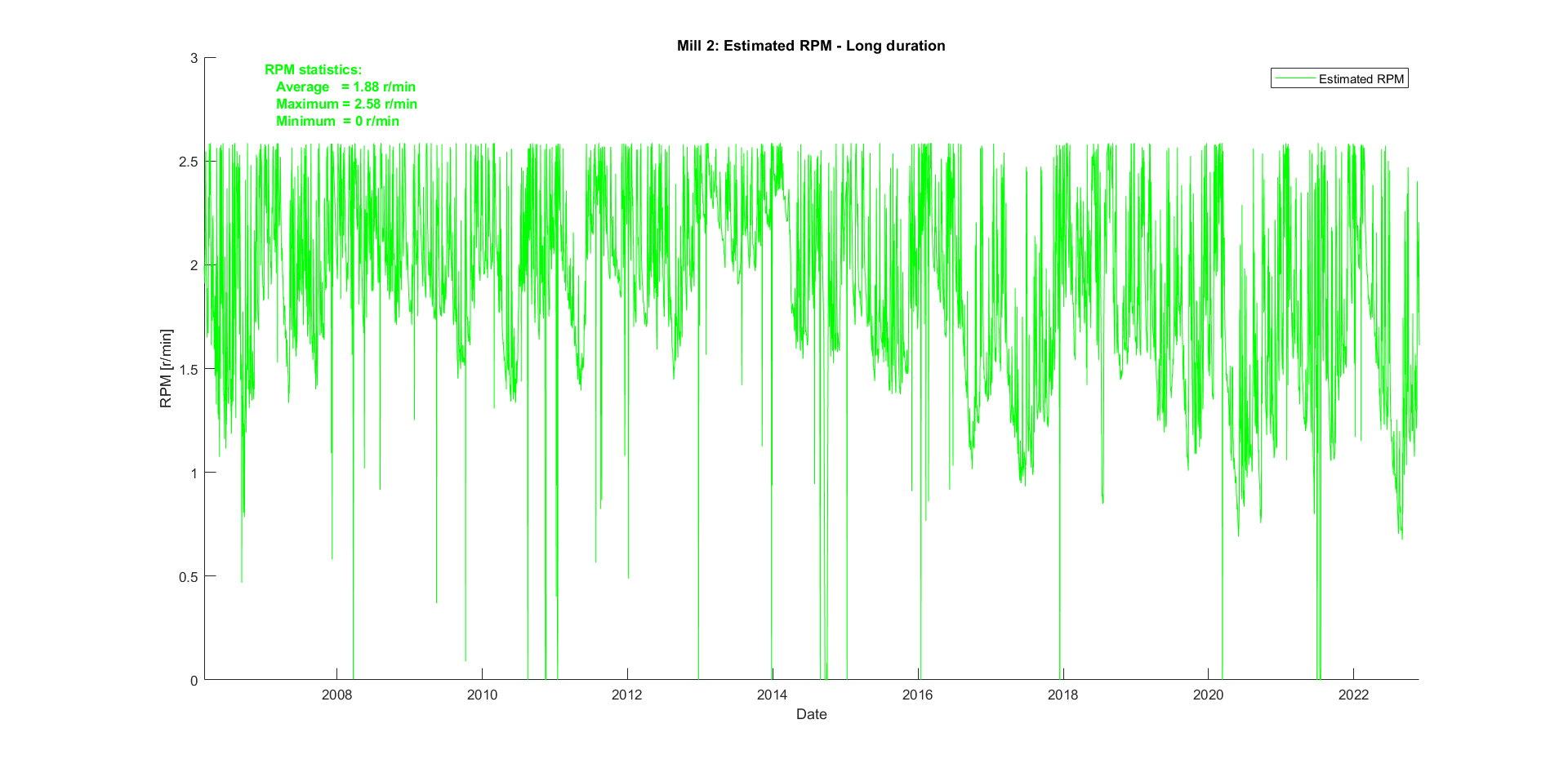
Zooming in again shows that the model fits the actual data quite well, as there is a single overpowering bin.